Model fitting • capturetb

library(ggplot2)
library(gridExtra)
library(dplyr)

This vignette demonstrates how the unitcost, unitcost_fixed and unitcost_ohd models were fitted and sensitivity analyses performed. It also shows how models could be fit using different covariates, target variable, training data or priors.

The following functions were included in the package to make the process of model development transparent and reproducible, but if you want to use the final capturetb models to predict costs you should read vignette("01_unitcost-model-predictions") and vignette("02_combining-predictions-data") instead.

Creating a model instance

A model instance requires a list of covariates, a target variable to predict, training data, and priors for parameters.

covariates <- c("logVisits", "logVisitsPP", "logVisitsPP_TB", "urban", "public")

target <- "ID_unitcost_total"

# Specifying priors for the fixed effects
# One beta coefficient for each covariate
# Other parameters will take default values
priors <- capturetb::capturetb_priors(
  beta.mean = rep(0, length(covariates)),
  beta.precision = rep(0.01, length(covariates))
)

data <- capturetb::get_data(output_name = "op_diagnosticvisit") 
# or provide your own data;
# see capturetb::outputs() for all output data 
# installed with the package

We now create an instance of the capturetb::JAGSModel class to fit a model with fixed covariate effects and country level random effects. If the data provided has more than one unique output type in the output column, the model will include facility and visit type effects. If the data has only one unique output type, no facility or visit type effects will be included.

model <- capturetb::JAGSModel$new(
  dat = data,
  covariates = covariates,
  target = target,
  priors = priors
)
#> Warning in initialize(...): Removed 3 rows with missing data.
#> Single output type detected. Not including output-level random effects in model.

Priors can be visualised by calling plot(priors, par = "name_of_param"):

priors <- model$priors()
plots <- list()
for(i in 1:3) {
  plots[[i]] <- plot(priors, par = paste0("beta[", i, "]"))
}
plots[[4]] <- plot(priors, par = "sigma_c")
plots[[5]] <- plot(priors, par = "sigma")
do.call(grid.arrange, c(plots, ncol = 3))
#> Warning: Removed 3341 rows containing missing values or values outside the scale range
#> (`geom_line()`).
#> Removed 3341 rows containing missing values or values outside the scale range
#> (`geom_line()`).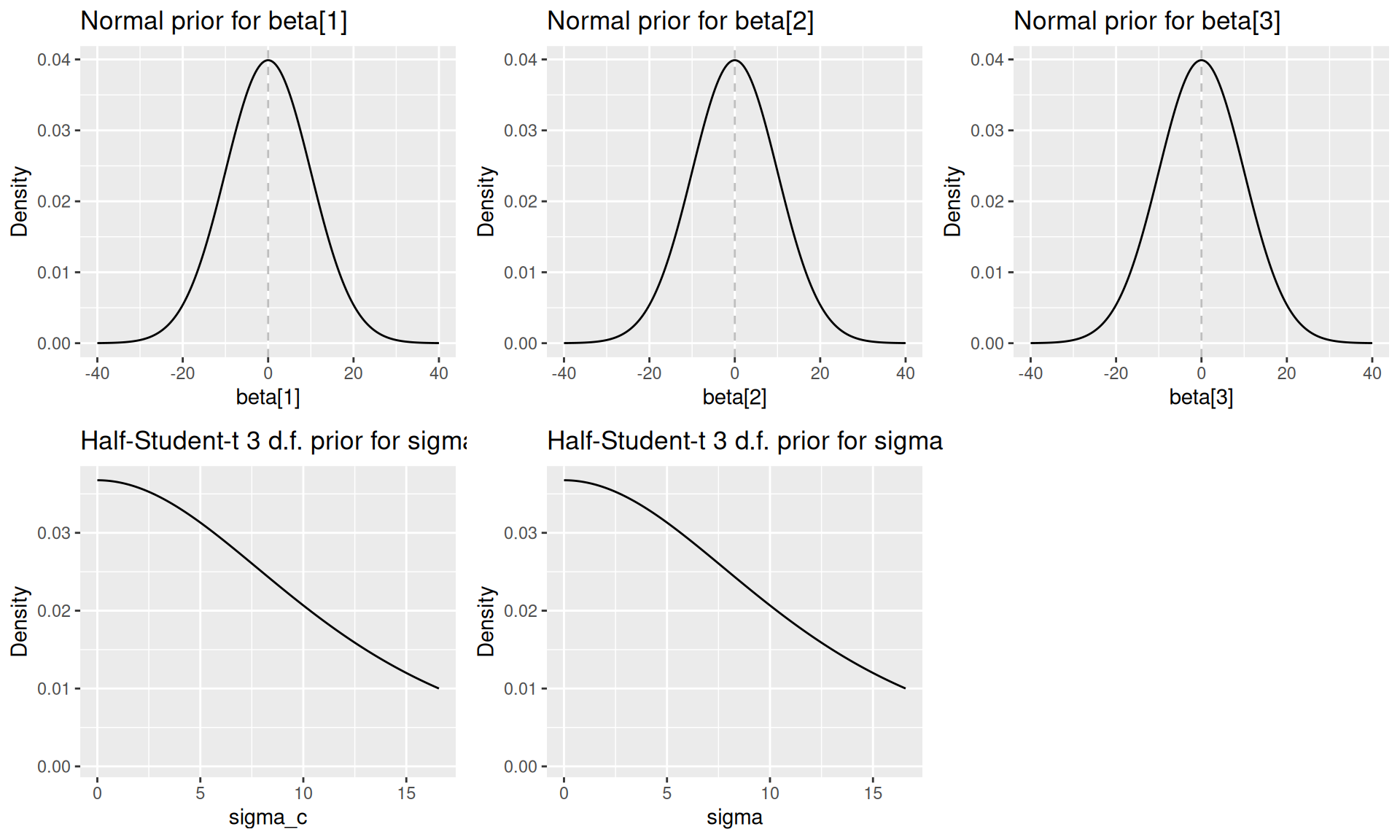

Fitting the model

Under the hood the JAGSModel class uses JAGS (Just Another Gibbs Sampler) to fit a multilevel linear regression model. To fit the model, JAGS and the runjags package must be installed on your machine.

For the purpose of the vignette, we’ll use fewer iterations than recommended for faster computation:

# Fit the model with reduced iterations for demonstration
# In practice, you might want to use the defaults (n.iter = 100000)
model$fit(
 n.iter = 20000,
 n.burnin = 1000,
 n.thin = 5,
 n.chains = 2
)

# Check summary statistics of the fitted samples
fitted_samples <- model$samples()
summary(fitted_samples)
#> 
#> Iterations = 6001:25996
#> Thinning interval = 5 
#> Number of chains = 2 
#> Sample size per chain = 4000 
#> 
#> 1. Empirical mean and standard deviation for each variable,
#>    plus standard error of the mean:
#> 
#>                       Mean      SD  Naive SE Time-series SE
#> alpha              3.68629 0.58188 0.0065057      0.0410492
#> beta[1]           -0.08047 0.05099 0.0005701      0.0033888
#> beta[2]            0.04320 0.05502 0.0006151      0.0007218
#> beta[3]           -0.35695 0.09523 0.0010647      0.0022346
#> beta[4]            0.39335 0.13803 0.0015432      0.0022879
#> beta[5]           -0.31483 0.12787 0.0014296      0.0017749
#> sigma              0.56500 0.04076 0.0004558      0.0004617
#> sigma_c            0.56452 0.42017 0.0046977      0.0220015
#> country_effect[1] -0.08318 0.34268 0.0038313      0.0185626
#> country_effect[2] -0.02249 0.35282 0.0039446      0.0185414
#> country_effect[3] -0.51342 0.35341 0.0039512      0.0183493
#> country_effect[4]  0.42390 0.34093 0.0038117      0.0174279
#> country_effect[5]  0.03346 0.35189 0.0039343      0.0211756
#> 
#> 2. Quantiles for each variable:
#> 
#>                       2.5%       25%        50%      75%    97.5%
#> alpha              2.58601  3.299015  3.6837600  4.05291  4.84284
#> beta[1]           -0.17788 -0.117171 -0.0796534 -0.04495  0.01802
#> beta[2]           -0.06425  0.006034  0.0430269  0.08034  0.14979
#> beta[3]           -0.54305 -0.419847 -0.3563490 -0.29284 -0.17202
#> beta[4]            0.12401  0.303090  0.3923715  0.48653  0.67127
#> beta[5]           -0.56765 -0.402291 -0.3129220 -0.23031 -0.06726
#> sigma              0.49229  0.536634  0.5631550  0.59075  0.65104
#> sigma_c            0.19775  0.335338  0.4513220  0.65862  1.61462
#> country_effect[1] -0.78192 -0.224156 -0.0585229  0.10022  0.46912
#> country_effect[2] -0.78336 -0.166740  0.0003765  0.16845  0.56450
#> country_effect[3] -1.26855 -0.654528 -0.4778230 -0.31345  0.03308
#> country_effect[4] -0.23707  0.270176  0.4351590  0.60398  1.03674
#> country_effect[5] -0.69461 -0.120335  0.0499534  0.22187  0.64314

Diagnostics

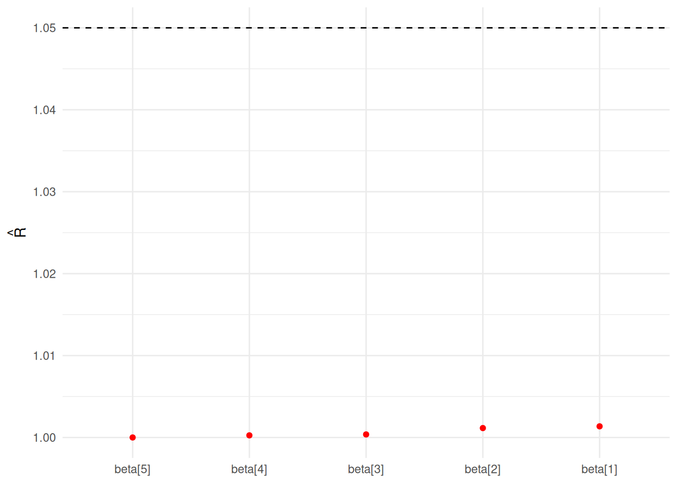
Several functions are available on the model class to check whether the model has converged:

Rhat:

model$mcmc_rhat(par = paste0("beta[", 1:length(covariates), "]"))

Trace:

model$mcmc_trace(regex_pars = "beta")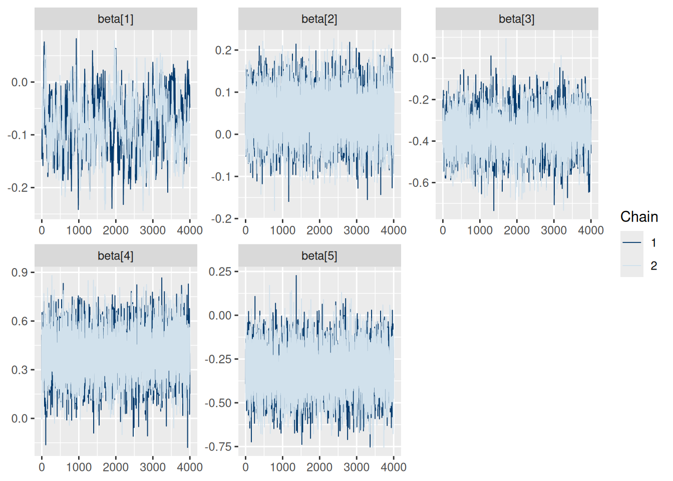

Auto-correlation:

model$mcmc_acf(regex_pars = "beta")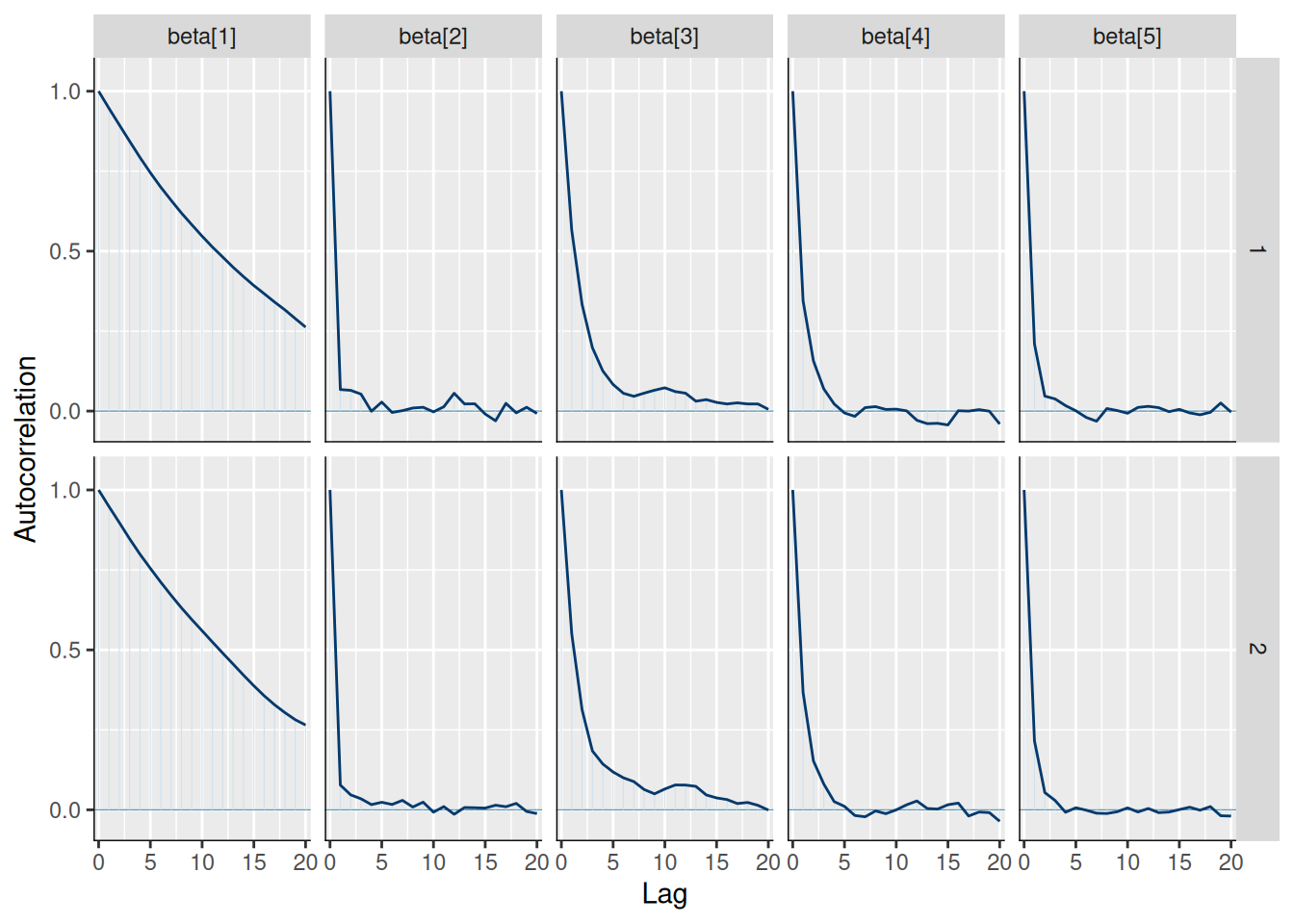

Effective sample size:

knitr::kable(model$n_eff())

	x
alpha	203.7431
beta[1]	226.3186
beta[2]	5807.3056
beta[3]	1875.6292
beta[4]	3640.0941
beta[5]	5190.2854
sigma	7799.8889
sigma_c	790.7373
country_effect[1]	453.7134
country_effect[2]	449.0084
country_effect[3]	541.0023
country_effect[4]	562.3751
country_effect[5]	434.5328

We can also plot the posterior distributions of each parameter:

model$plot_posteriors(pars = paste0("beta[", 1:length(covariates), "]")) + 
  ggplot2::scale_y_discrete(labels = covariates)
#> Scale for y is already present.
#> Adding another scale for y, which will replace the existing scale.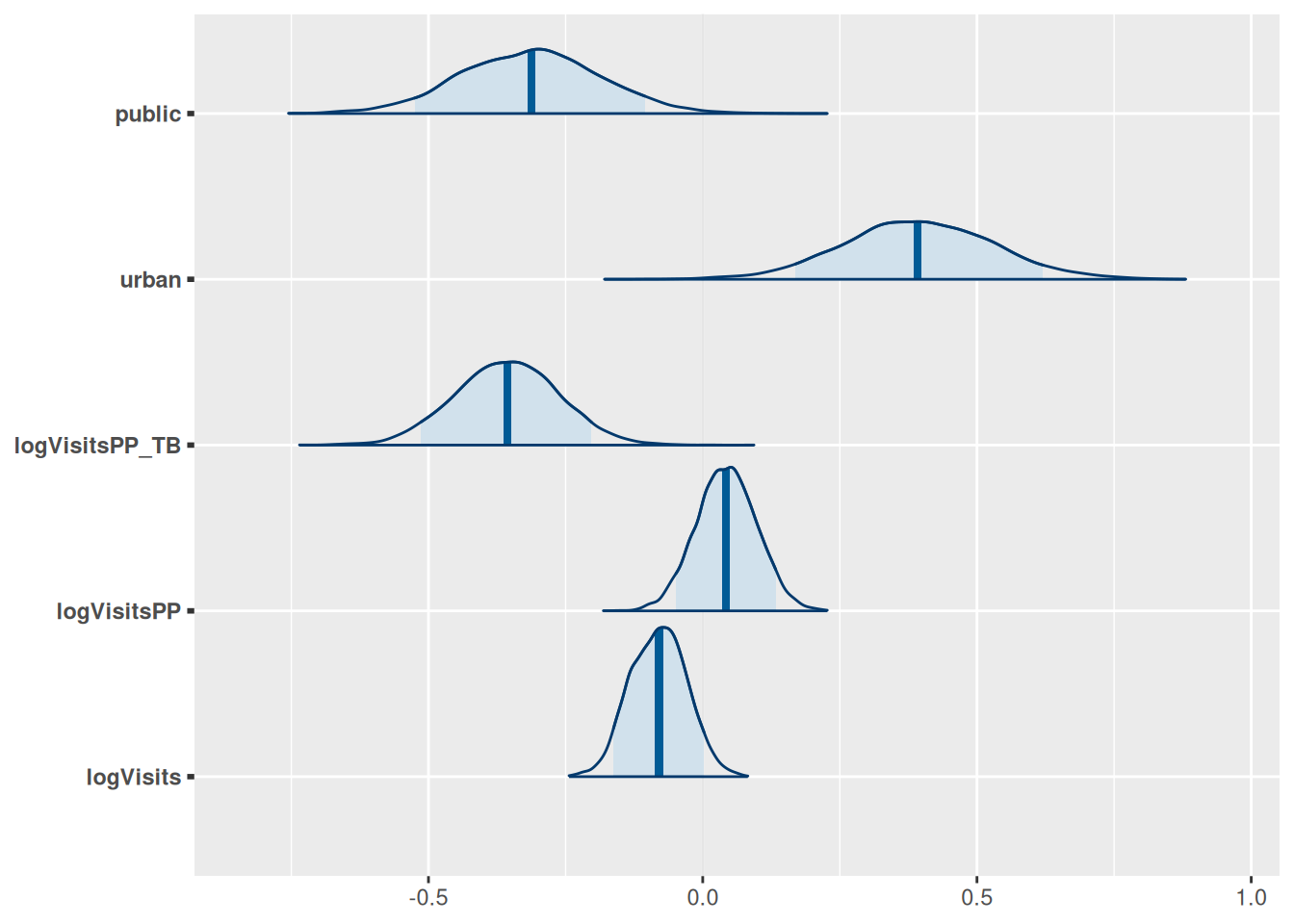

model$plot_posteriors(pars = paste0("country_effect[", 1:5, "]"))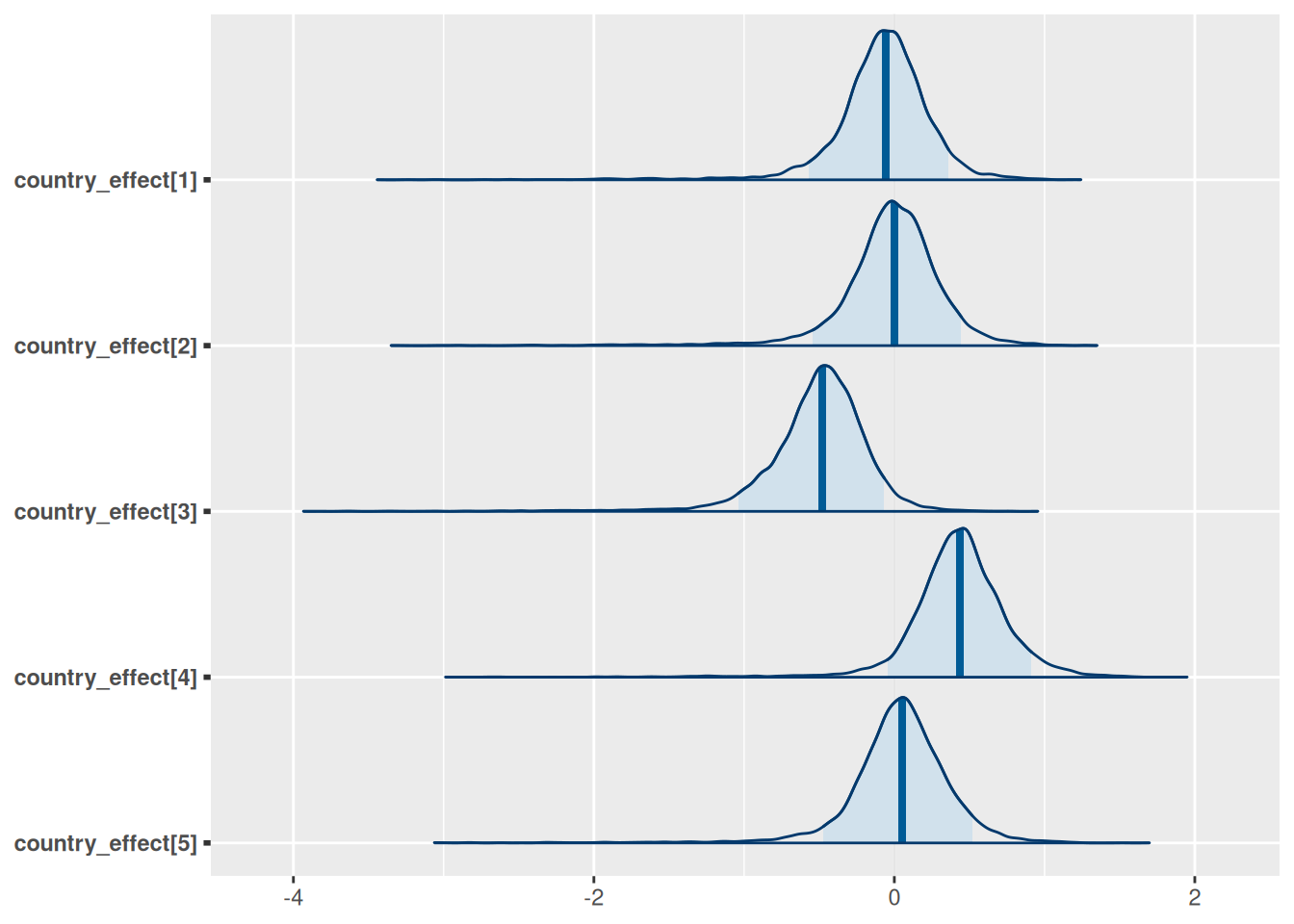

Generating predictions

We can now generate predictions for the training data and evaluate model fit:

# Generate predictions for the training data on log scale
dat <- model$training_data()
predictions <- model$predict(dat, scale = "log", summarised = TRUE)
head(predictions)
#> Summary of Posterior Distribution
#> 
#> Observation | Mean |       95% CI
#> ---------------------------------
#> 1           | 3.47 | [2.28, 4.65]
#> 2           | 2.67 | [1.52, 3.84]
#> 3           | 2.08 | [0.89, 3.23]
#> 4           | 1.84 | [0.67, 3.02]
#> 5           | 2.25 | [1.10, 3.39]
#> 6           | 2.27 | [1.14, 3.40]

# Various measures of fit
performance <- model$performance(scale = "log")
knitr::kable(performance)

mae	rmse	ci_coverage	median_ci	bayesian_r2
0.4324535	0.53582	0.9716981	2.319828	0.4984564

Visualising results

1. Predicted vs Observed

# Create scatter plot of predicted vs observed values
model$plot_fit(include_ci = FALSE, scale = "log")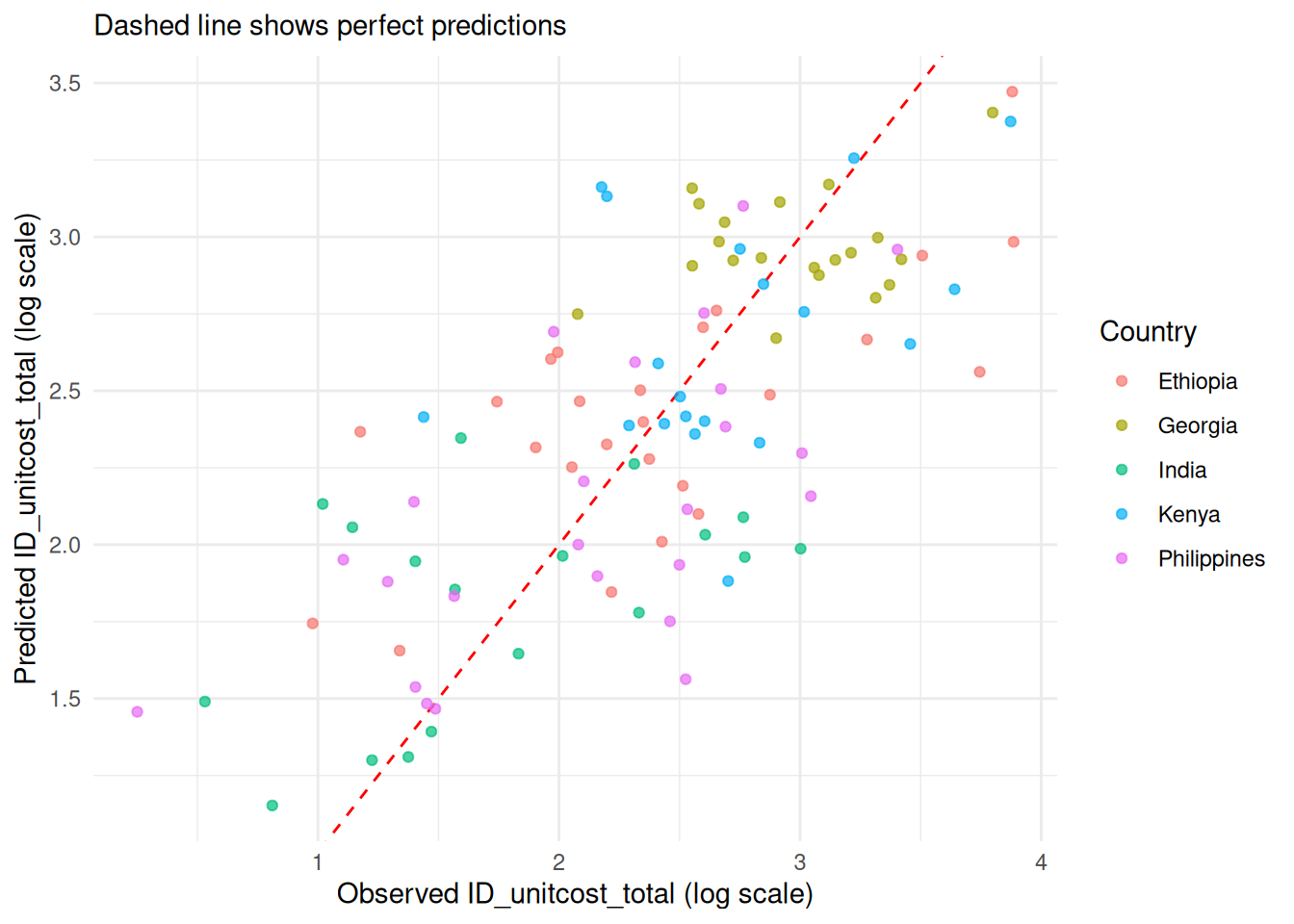

2. 95% Credible Prediction Intervals

# Plot with prediction intervals
model$plot_fit(include_ci = TRUE, scale = "log")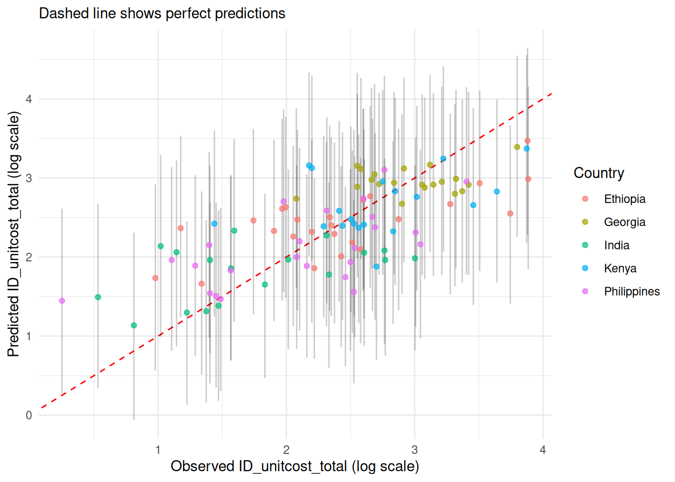

3. Residuals

model$plot_residuals(add_smooth = TRUE, color_by_country = TRUE)
#> Warning in private$.predict(dat, include_epsilon = FALSE, conditional = TRUE):
#> conditional = TRUE has no effect when there is only one output type
#> `geom_smooth()` using formula = 'y ~ x'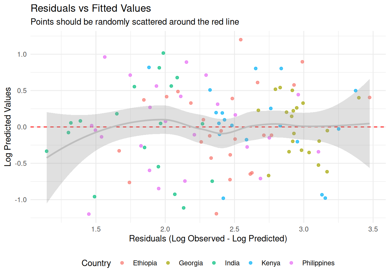

4. Country-Specific perfomance

# Performance by country
country_performance <- model$performance(by_country = TRUE)
colnames(country_performance) <- c("Country", "MAE",
 "RMSE", "95% CI Coverage", "Median CI Width", "Bayesian R-squ")

knitr::kable(country_performance)

Country	MAE	RMSE	95% CI Coverage	Median CI Width	Bayesian R-squ
Ethiopia	6.905357	9.392090	0.9200000	33.95291	0.3961824
Georgia	6.810341	8.027912	1.0000000	53.73618	0.4403003
India	3.920241	4.998105	1.0000000	20.81572	0.3554724
Kenya	7.021894	9.399381	1.0000000	38.53299	0.4302563
Philippines	4.542880	5.554474	0.9583333	22.58788	0.4842272

model$plot_fit() + 
  ggplot2::facet_wrap(~country, scales = "free")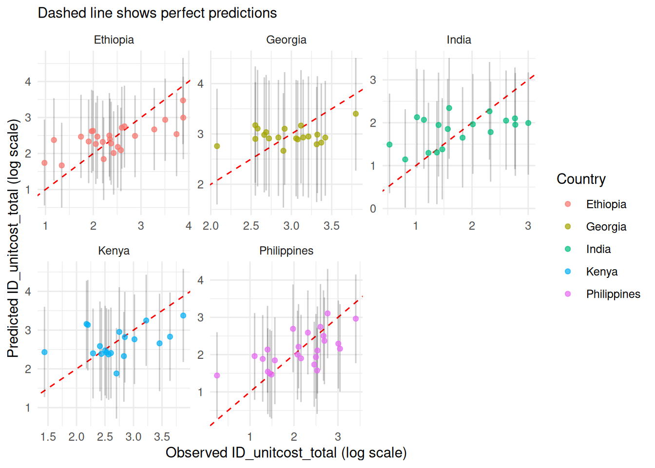

5. Out-of-sample performance

We can check for overfitting and estimate out-of-sample performance using k-fold cross-validation. Here we use 3 folds for quick compilation; in practice, 10 or 20 folds would give a more accurate picture.

res <- model$k_fold_cv(k_folds = 3, 
  n.iter = 10000,
  n.burnin = 1000,
  n.adapt = 1000, 
  scale = "log")
#> Processing fold 1 of 3
#> Single output type detected. Not including output-level random effects in model.
#> Calling 3 simulations using the parallel method...
#> Following the progress of chain 1 (the program will wait for all chains
#> to finish before continuing):
#> Welcome to JAGS 4.3.2 on Thu Dec 11 11:19:52 2025
#> JAGS is free software and comes with ABSOLUTELY NO WARRANTY
#> Loading module: basemod: ok
#> Loading module: bugs: ok
#> . . Reading data file data.txt
#> . Compiling model graph
#>    Resolving undeclared variables
#>    Allocating nodes
#> Graph information:
#>    Observed stochastic nodes: 70
#>    Unobserved stochastic nodes: 83
#>    Total graph size: 879
#> . Reading parameter file inits1.txt
#> . Initializing model
#> . Adapting 1000
#> -------------------------------------------------| 1000
#> ++++++++++++++++++++++++++++++++++++++++++++++++++ 100%
#> Adaptation successful
#> . Updating 1000
#> -------------------------------------------------| 1000
#> ************************************************** 100%
#> . . . . . . Updating 10000
#> -------------------------------------------------| 10000
#> ************************************************** 100%
#> . . . . Updating 0
#> . Deleting model
#> . 
#> All chains have finished
#> Simulation complete.  Reading coda files...
#> Coda files loaded successfully
#> Finished running the simulation
#> Compiling rjags model and adapting for 1000 iterations...
#> Obtaining DIC samples from 100 iterations...
#> Model fitted successfully with 3 chains and 10000 iterations.
#> Processing fold 2 of 3
#> Single output type detected. Not including output-level random effects in model.
#> Calling 3 simulations using the parallel method...
#> Following the progress of chain 1 (the program will wait for all chains
#> to finish before continuing):
#> Welcome to JAGS 4.3.2 on Thu Dec 11 11:19:53 2025
#> JAGS is free software and comes with ABSOLUTELY NO WARRANTY
#> Loading module: basemod: ok
#> Loading module: bugs: ok
#> . . Reading data file data.txt
#> . Compiling model graph
#>    Resolving undeclared variables
#>    Allocating nodes
#> Graph information:
#>    Observed stochastic nodes: 71
#>    Unobserved stochastic nodes: 84
#>    Total graph size: 891
#> . Reading parameter file inits1.txt
#> . Initializing model
#> . Adapting 1000
#> -------------------------------------------------| 1000
#> ++++++++++++++++++++++++++++++++++++++++++++++++++ 100%
#> Adaptation successful
#> . Updating 1000
#> -------------------------------------------------| 1000
#> ************************************************** 100%
#> . . . . . . Updating 10000
#> -------------------------------------------------| 10000
#> ************************************************** 100%
#> . . . . Updating 0
#> . Deleting model
#> . 
#> All chains have finished
#> Simulation complete.  Reading coda files...
#> Coda files loaded successfully
#> Finished running the simulation
#> Compiling rjags model and adapting for 1000 iterations...
#> Obtaining DIC samples from 100 iterations...
#> Model fitted successfully with 3 chains and 10000 iterations.
#> Processing fold 3 of 3
#> Single output type detected. Not including output-level random effects in model.
#> Calling 3 simulations using the parallel method...
#> Following the progress of chain 1 (the program will wait for all chains
#> to finish before continuing):
#> Welcome to JAGS 4.3.2 on Thu Dec 11 11:19:54 2025
#> JAGS is free software and comes with ABSOLUTELY NO WARRANTY
#> Loading module: basemod: ok
#> Loading module: bugs: ok
#> . . Reading data file data.txt
#> . Compiling model graph
#>    Resolving undeclared variables
#>    Allocating nodes
#> Graph information:
#>    Observed stochastic nodes: 71
#>    Unobserved stochastic nodes: 84
#>    Total graph size: 891
#> . Reading parameter file inits1.txt
#> . Initializing model
#> . Adapting 1000
#> -------------------------------------------------| 1000
#> ++++++++++++++++++++++++++++++++++++++++++++++++++ 100%
#> Adaptation successful
#> . Updating 1000
#> -------------------------------------------------| 1000
#> ************************************************** 100%
#> . . . . . . Updating 10000
#> -------------------------------------------------| 10000
#> ************************************************** 100%
#> . . . . Updating 0
#> . Deleting model
#> . 
#> All chains have finished
#> Simulation complete.  Reading coda files...
#> Coda files loaded successfully
#> Finished running the simulation
#> Compiling rjags model and adapting for 1000 iterations...
#> Obtaining DIC samples from 100 iterations...
#> Model fitted successfully with 3 chains and 10000 iterations.

fit <- res |> 
  group_by(fold) |> 
  summarise(rmse = sqrt(mean((observed-mean)^2)),
            mae = mean(abs(observed-mean)))

knitr::kable(fit)

fold	rmse	mae
1	0.6549080	0.5502908
2	0.5967717	0.4598268
3	0.6183338	0.5211409

Reproducing the fitted models installed with the package

There are three pre-fitted models installed with the package:

unitcost(): predicts the cost of a single outpatient visit
unitcost_fixed(): predicts the fixed costs associated with a single outpatient visit
unitcost_ohd(): predicts the fixed costs associated with a single outpatient visit

mod_unit <- unitcost()
mod_unit$fit(seed = 1)
samples <- mod_unit$samples()
DIC <- mod_unit$mcmc_DIC(summarised = FALSE)
saveRDS(samples, "inst/posterior_samples.rds")
saveRDS(DIC, "inst/posterior_samples_dic.rds")

mod_unit_fixed <- unitcost_fixed()
mod_unit_fixed$fit(seed = 1)
samples_fixed <- mod_unit_fixed$samples()
DIC <- mod_unit$mcmc_DIC(summarised = FALSE)
saveRDS(samples_fixed, "inst/posterior_samples_fixed.rds")
saveRDS(DIC_fixed, "inst/posterior_samples_dic_fixed.rds")

mod_unit_ohd <- unitcost_ohd()
mod_unit_ohd$fit(seed = 1)
samples_ohd <- mod_unit_ohd$samples()
DIC_ohd <- mod_unit_ohd$mcmc_DIC(summarised = FALSE)
saveRDS(samples_ohd, "inst/posterior_samples_ohd.rds")
saveRDS(DIC_ohd, "inst/posterior_samples_dic_ohd.rds")

Executing the above code will reproduce exactly the posterior samples installed with this package. The functions unitcost(), unitcost_fixed() and unitcost_ohd() use the saved posteriors to load the models without requiring fitting at runtime.